Generalized linear model

Not to be confused with general linear model or generalized least squares.

In statistics, the generalized linear model (GLM) is a flexible generalization of ordinary linear regression. The GLM generalizes linear regression by allowing the linear model to be related to the response variable via a link function and by allowing the magnitude of the variance of each measurement to be a function of its predicted value.

Generalized linear models were formulated by John Nelder and Robert Wedderburn as a way of unifying various other statistical models, including linear regression, logistic regression and Poisson regression.^[1] They proposed an iteratively reweighted least squares method for maximum likelihood estimation of the model parameters. Maximum-likelihood estimation remains popular and is the default method on many statistical computing packages. Other approaches, including Bayesian approaches and least squares fits to variance stabilized responses, have been developed.

Overview

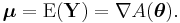
In a GLM, each outcome of the dependent variables, Y, is assumed to be generated from a particular distribution in the exponential family, a large range of probability distributions that includes the normal, binomial and poisson distributions, among others. The mean, μ, of the distribution depends on the independent variables, X, through:

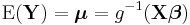
$\operatorname{E}(\mathbf{Y}) = \boldsymbol{\mu} = g^{-1}(\mathbf{X}\boldsymbol{\beta})$

where E(Y) is the expected value of Y; Xβ is the linear predictor, a linear combination of unknown parameters, β; g is the link function.

In this framework, the variance is typically a function, V, of the mean:

$\operatorname{Var}(\mathbf{Y}) = \operatorname{V}( \boldsymbol{\mu} ) = \operatorname{V}(g^{-1}(\mathbf{X}\boldsymbol{\beta})).$

It is convenient if V follows from the exponential family distribution, but it may simply be that the variance is a function of the predicted value.

The unknown parameters, β, are typically estimated with maximum likelihood, maximum quasi-likelihood, or Bayesian techniques.

Model components

The GLM consists of three elements:

1. A probability distribution from the exponential family.

2. A linear predictor η = Xβ .

3. A link function g such that E(Y) = μ = g^-1(η).

Probability distribution

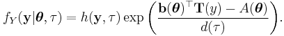
The overdispersed exponential family of distributions is a generalization of the exponential family and exponential dispersion model of distributions and includes those probability distributions, parameterized by $\boldsymbol\theta$ and $\tau$ , whose density functions f (or probability mass function, for the case of a discrete distribution) can be expressed in the form

$f_Y(\mathbf{y} | \boldsymbol\theta, \tau) = h(\mathbf{y},\tau) \exp{\left(\frac{\mathbf{b}(\boldsymbol\theta)^{\top}\mathbf{T}(y) - A(\boldsymbol\theta)} {d(\tau)} \right)}. \,\!$

$\tau$ , called the dispersion parameter, typically is known and is usually related to the variance of the distribution. The functions $h(\mathbf{y},\tau)$ , $\mathbf{b}(\boldsymbol\theta)$ , $\mathbf{T}(y)$ , $A(\boldsymbol\theta)$ , and $d(\tau)$ are known. Many, although not all, common distributions are in this family.

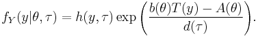
For scalar $Y$ and $\theta$ , this reduces to

$f_Y(y | \theta, \tau) = h(y,\tau) \exp{\left(\frac{b(\theta)T(y) - A(\theta)}{d(\tau)} \right)}. \,\!$

$\boldsymbol\theta$ is related to the mean of the distribution. If $\mathbf{b}(\boldsymbol\theta)$ is the identity function, then the distribution is said to be in canonical form (or natural form). Note that any distribution can be converted to canonical form by rewriting $\boldsymbol\theta$ as $\boldsymbol\theta'$ and then applying the transformation $\boldsymbol\theta = \mathbf{b}(\boldsymbol\theta')$ . It is always possible to convert $A(\boldsymbol\theta)$ in terms of the new parametrization, even if $\mathbf{b}(\boldsymbol\theta')$ is not a one-to-one function; see comments in the page on the exponential family. If, in addition, $\mathbf{T}(y)$ is the identity and $\tau$ is known, then $\boldsymbol\theta$ is called the canonical parameter (or natural parameter) and is related to the mean through

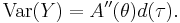
$\boldsymbol\mu = \operatorname{E}(\mathbf{Y}) = \nabla A(\boldsymbol\theta). \,\!$

For scalar $Y$ and $\theta$ , this reduces to

$\mu = \operatorname{E}(Y) = A'(\theta). \,\!$

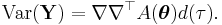
Under this scenario, the variance of the distribution can be shown to be^[2]

$\operatorname{Var}(\mathbf{Y}) = \nabla\nabla^{\top} A(\boldsymbol\theta) d(\tau). \,\!$

For scalar $Y$ and $\theta$ , this reduces to

$\operatorname{Var}(Y) = A''(\theta) d(\tau). \,\!$

Linear predictor

The linear predictor is the quantity which incorporates the information about the independent variables into the model. The symbol η (Greek "eta") is typically used to denote a linear predictor. It is related to the expected value of the data (thus, "predictor") through the link function.

η is expressed as linear combinations (thus, "linear") of unknown parameters β. The coefficients of the linear combination are represented as the matrix of independent variables X. η can thus be expressed as

$\eta = \mathbf{X}\boldsymbol{\beta}.\,$

The elements of X are either measured by the experimenters or stipulated by them in the modeling design process.

Link function

The link function provides the relationship between the linear predictor and the mean of the distribution function. There are many commonly used link functions, and their choice can be somewhat arbitrary. It can be convenient to match the domain of the link function to the range of the distribution function's mean.

When using a distribution function with a canonical parameter $\theta$ , the canonical link function is the function that expresses $\theta$ in terms of $\mu$ , i.e. $\theta = b(\mu)$ . For the most common distributions, the mean $\mu$ is one of the parameters in the standard form of the distribution's density function, and then $b(\mu)$ is the function as defined above that maps the density function into its canonical form. When using the canonical link function, $b(\mu) = \theta = \mathbf{X}\boldsymbol{\beta}$ , which allows $\mathbf{X}^T \mathbf{Y}$ to be a sufficient statistic for $\boldsymbol{\beta}$ .

Following is a table of canonical link functions and their inverses (sometimes referred to as the mean function, as done here) used for several distributions in the exponential family.

Canonical Link Functions
Distribution	Name	Link Function	Mean Function
Normal	Identity	$\mathbf{X}\boldsymbol{\beta}=\mu\,\!$	$\mu=\mathbf{X}\boldsymbol{\beta}\,\!$
Exponential	Inverse	$\mathbf{X}\boldsymbol{\beta}=\mu^{-1}\,\!$	$\mu=(\mathbf{X}\boldsymbol{\beta})^{-1}\,\!$
Gamma	Inverse	$\mathbf{X}\boldsymbol{\beta}=\mu^{-1}\,\!$	$\mu=(\mathbf{X}\boldsymbol{\beta})^{-1}\,\!$
Inverse Gaussian	Inverse squared	$\mathbf{X}\boldsymbol{\beta}=\mu^{-2}\,\!$	$\mu=(\mathbf{X}\boldsymbol{\beta})^{-1/2}\,\!$
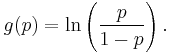
Poisson	Log	$\mathbf{X}\boldsymbol{\beta}=\ln{(\mu)}\,\!$	$\mu=\exp{(\mathbf{X}\boldsymbol{\beta})}\,\!$
Binomial	Logit	$\mathbf{X}\boldsymbol{\beta}=\ln{\left(\frac{\mu}{1-\mu}\right)}\,\!$	$\mu=\frac{\exp{(\mathbf{X}\boldsymbol{\beta})}}{1 %2B \exp{(\mathbf{X}\boldsymbol{\beta})}} = \frac{1}{1 %2B \exp{(-\mathbf{X}\boldsymbol{\beta})}}\,\!$
Multinomial	Logit

In the cases of the exponential and gamma distributions, the domain of the canonical link function is not the same as the permitted range of the mean. In particular, the linear predictor may be negative, which would give an impossible negative mean. When maximizing the likelihood, precautions must be taken to avoid this. An alternative is to use a noncanonical link function.

Fitting

Maximum likelihood

The maximum likelihood estimates can be found using an iteratively reweighted least squares algorithm using either a Newton–Raphson method with updates of the form:

$\boldsymbol\beta^{(t%2B1)} = \boldsymbol\beta^{(t)} %2B \mathcal{J}^{-1}(\boldsymbol\beta^{(t)}) u(\boldsymbol\beta^{(t)}),$

where $\mathcal{J}(\boldsymbol\beta^{(t)})$ is the observed information matrix (the negative of the Hessian matrix) and $u(\boldsymbol\beta^{(t)})$ is the score function; or a Fisher's scoring method:

$\boldsymbol\beta^{(t%2B1)} = \boldsymbol\beta^{(t)} %2B \mathcal{I}^{-1}(\boldsymbol\beta^{(t)}) u(\boldsymbol\beta^{(t)}),$

where $\mathcal{I}(\boldsymbol\beta^{(t)})$ is the Fisher information matrix. Note that if the canonical link function is used, then the two methods are the same.^[3]

Bayesian methods

In general, the posterior distribution cannot be found in closed form and so must be approximated, usually using Laplace approximations or some type of Markov chain Monte Carlo method such as Gibbs sampling.

Examples

General linear models

A possible point of confusion has to do with the distinction between generalized linear models and the general linear model, two broad statistical models. The general linear model may be viewed as a case of the generalized linear model with identity link. As most exact results of interest are obtained only for the general linear model, the general linear model has undergone a somewhat longer historical development. Results for the generalized linear model with non-identity link are asymptotic (tending to work well with large samples).

Linear regression

A simple, very important example of a generalized linear model (also an example of a general linear model) is linear regression. In linear regression, the use of the least-squares estimator is justified by the Gauss-Markov theorem, which does not assume that the distribution is normal.

From the perspective of generalized linear models, however, it is useful to suppose that the distribution function is the normal distribution with constant variance and the link function is the identity, which is the canonical link if the variance is known.

For the normal distribution, the generalized linear model has a closed form expression for the maximum-likelihood estimates, which is convenient. Most other GLMs lack closed form estimates.

Binomial data

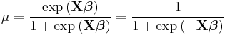
When the response data, Y, are binary (taking on only values 0 and 1), the distribution function is generally chosen to be the binomial distribution and the interpretation of μ_i is then the probability, p, of Y_i taking on the value one.

There are several popular link functions for binomial functions; the most typical is the canonical logit link:

$g(p) = \ln \left( { p \over 1-p } \right).$

GLMs with this setup are logistic regression models.

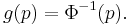
In addition, the inverse of any continuous cumulative distribution function (CDF) can be used for the link since the CDF's range is $[0,1]$ , the range of the binomial mean. The normal CDF $\Phi$ is a popular choice and yields the probit model. Its link is

$g(p) = \Phi^{-1}(p).\,\!$

The complementary log-log function $log(-log(1- p))$ may also be used. This link function is asymmetric and will often produce different results from the probit and logit link functions.

The identity link is also sometimes used for binomial data to yield the linear probability model, but a drawback of this model is that the predicted probabilities can be greater than one or less than zero. In implementation it is possible to fix the nonsensical probabilities outside of $[0,1]$ , but interpreting the coefficients can be difficult. The model's primary merit is that near $p = 0.5$ it is approximately a linear transformation of the probit and logit―econometricians sometimes call this the Harvard model.

The variance function for binomial data is given by:

$\operatorname{Var}(Y_{i})= \tau\mu_{i} (1-\mu_{i})\,\!$

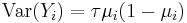
where the dispersion parameter τ is typically fixed at exactly one. When it is not, the resulting quasi-likelihood model often described as binomial with overdispersion or quasibinomial.

Count data

Another example of generalized linear models includes Poisson regression which models count data using the Poisson distribution. The link is typically the logarithm, the canonical link.

The variance function is proportional to the mean

$\operatorname{var}(Y_{i}) = \tau\mu_{i},\,$

where the dispersion parameter τ is typically fixed at exactly one. When it is not, the resulting quasi-likelihood model is often described as poisson with overdispersion or quasipoisson.

Extensions

Correlated or clustered data

The standard GLM assumes that the observations are uncorrelated. Extensions have been developed to allow for correlation between observations, as occurs for example in longitudinal studies and clustered designs:

Generalized estimating equations (GEEs) allow for the correlation between observations without the use of an explicit probability model for the origin of the correlations, so there is no explicit likelihood. They are suitable when the random effects and their variances are not of inherent interest, as they allow for the correlation without explaining its origin. The focus is on estimating the average response over the population ("population-averaged" effects) rather than the regression parameters that would enable prediction of the effect of changing one or more components of X on a given individual. GEEs are usually used in conjunction with Huber-White standard errors.^[4]^[5]
Generalized linear mixed models (GLMMs) are an extension to GLMs that includes random effects in the linear predictor, giving an explicit probability model that explains the origin of the correlations. The resulting "subject-specific" parameter estimates are suitable when the focus is on estimating the effect of changing one or more components of X on a given individual. GLMMs are a particular type of multilevel model (mixed model). In general, fitting GLMMs is more computationally complex and intensive than fitting GEEs.
Hierarchical generalized linear models (HGLMs) are similar to GLMMs apart from two distinctions:

The random effects can have any distribution in the exponential family, whereas current GLMMs nearly always have normal random effects;
They are not as computationally intensive, as instead of integrating out the random effects they are based on a modified form of likelihood known as the hierarchical likelihood or h-likelihood.

The theoretical basis and accuracy of the methods used in HGLMs have been the subject of some debate in the statistical literature.^[6]

Generalized additive models

Generalized additive models (GAMs) are another extension to GLMs in which the linear predictor η is not restricted to be linear in the covariates X but is the sum of smoothing functions applied to the x_is:

$\eta = \beta_0 %2B f_1(x_1) %2B f_2(x_2) %2B \ldots \,\!$

The smoothing functions f_i are estimated from the data. In general this requires a large number of data points and is computationally intensive.^[7]^[8]

Multinomial regression

The binomial case may be easily extended to allow for a multinomial distribution as the response (also, a Generalized Linear Model for counts, with a constrained total). There are two ways in which this is usually done:

Ordered response

If the response variable is an ordinal measurement, then one may fit a model function of the form:

$g(\mu_m) = \eta_m = \beta_0 %2B X_1 \beta_1 %2B \ldots %2B X_p \beta_p %2B \gamma_2 %2B \ldots %2B \gamma_m = \eta_1 %2B \gamma_2 %2B \ldots %2B \gamma_m \,$ where $\mu_m = \mathrm{P}(Y \leq m) \,$ .

for m > 2. Different links g lead to proportional odds models or ordered probit models.

Unordered response

If the response variable is a nominal measurement, or the data do not satisfy the assumptions of an ordered model, one may fit a model of the following form:

$g(\mu_m) = \eta_m = \beta_{m,0} %2B X_1 \beta_{m,1} %2B \ldots %2B X_p \beta_{m,p} \,$ where $\mu_m = \mathrm{P}(Y = m \mid Y \in \{1,m\} ) \,$ .

for m > 2. Different links g lead to multinomial logit or multinomial probit models. These are less efficient than the ordered response models, as more parameters are estimated.

Confusion with general linear models

The term "generalized linear model", and especially its abbreviation GLM, can be confused with general linear model. John Nelder has expressed regret about this in a conversation with Stephen Senn:

Senn: I must confess to having some confusion when I was a young statistician between general linear models and generalized linear models. Do you regret the terminology?

Nelder: I think probably I do. I suspect we should have found some more fancy name for it that would have stuck and not been confused with the general linear model, although general and generalized are not quite the same. I can see why it might have been better to have thought of something else.^[9]

Notes

^ Nelder, John; Wedderburn, Robert (1972). "Generalized Linear Models". Journal of the Royal Statistical Society. Series A (General) (Blackwell Publishing) 135 (3): 370–384. doi:10.2307/2344614. JSTOR 2344614.
^ McCullagh and Nelder (1989), Chapter 2.
^ McCullagh and Nelder (1989), Page 43.
^ Zeger, Scott L.; Liang, Kung-Yee; Albert, Paul S. (1988). "Models for Longitudinal Data: A Generalized Estimating Equation Approach". Biometrics (International Biometric Society) 44 (4): 1049–1060. doi:10.2307/2531734. JSTOR 2531734. PMID 3233245.
^ Hardin, James; Hilbe, Joseph (2003). Generalized Estimating Equations. London: Chapman and Hall/CRC. ISBN 1584883073.
^ Lee, Youngjo; Nelder, John; Pawitan, Yudi (2006). Generalized Linear Models with Random Effects: Unified Analysis via H-likelihood. Chapman & Hall/CRC. ISBN 1584886315.
^ Hastie, T. J.; Tibshirani, R. J. (1990). Generalized Additive Models. Chapman & Hall/CRC. ISBN 9780412343902.
^ Wood, Simon (2006). Generalized Additive Models: An Introduction with R. Chapman & Hall/CRC. ISBN 1-584-88474-6.
^ Senn, Stephen (2003). "A conversation with John Nelder". Statistical Science 18 (1): 118–131. doi:10.1214/ss/1056397489. http://projecteuclid.org/euclid.ss/1056397489.

References

McCullagh, Peter; Nelder, John (1989). Generalized Linear Models, Second Edition. Boca Raton: Chapman and Hall/CRC. ISBN 0-412-31760-5.

External links

Statistics

Descriptive statistics

Continuous data

Location	Mean (Arithmetic, Geometric, Harmonic) Median Mode

Dispersion	Range Standard deviation Coefficient of variation Percentile Interquartile range

Shape	Variance Skewness Kurtosis Moments L-moments

Count data

Index of dispersion

Summary tables

Dependence

Statistical graphics

Data collection

Designing studies	Effect size Standard error Statistical power Sample size determination

Survey methodology	Sampling Stratified sampling Opinion poll Questionnaire

Controlled experiment	Design of experiments Randomized experiment Random assignment Replication Blocking Factorial experiment Optimal design

Uncontrolled studies	Natural experiment Quasi-experiment Observational study

Statistical inference

Statistical theory	Sampling distribution Sufficient statistic Meta-analysis

Bayesian inference	Bayesian probability Prior Posterior Credible interval Bayes factor Bayesian estimator Maximum posterior estimator

Frequentist inference	Confidence interval Hypothesis testing Likelihood-ratio

Specific tests	Z-test (normal) Student's t-test F-test Pearson's chi-squared test Wald test Mann–Whitney U Shapiro–Wilk Signed-rank Kolmogorov–Smirnov test

General estimation	Bias Robustness Efficiency Maximum likelihood Method of moments Minimum distance Density estimation

Correlation and regression analysis

Correlation	Pearson product-moment correlation Partial correlation Confounding variable Coefficient of determination

Regression analysis	Errors and residuals Regression model validation Mixed effects models Simultaneous equations models

Linear regression	Simple linear regression Ordinary least squares General linear model Bayesian regression

Non-standard predictors	Nonlinear regression Nonparametric Semiparametric Isotonic Robust

Generalized linear model	Exponential families Logistic (Bernoulli) Binomial Poisson

Partition of variance	Analysis of variance (ANOVA) Analysis of covariance Multivariate ANOVA Degrees of freedom

Categorical, multivariate, time-series, or survival analysis

Categorical data	Cohen's kappa Contingency table Graphical model Log-linear model McNemar's test

Multivariate statistics	Multivariate regression Principal components Factor analysis Cluster analysis Copulas

Time series analysis	Decomposition (Trend, Stationary process) ARMA model ARIMA model Vector autoregression Spectral density estimation

Survival analysis	Survival function Kaplan–Meier Logrank test Failure rate Proportional hazards models Accelerated failure time model

Applications

Biostatistics	Bioinformatics Biometrics Clinical trials & studies Epidemiology Medical statistics

Engineering statistics	Chemometrics Methods engineering Probabilistic design Process & Quality control Reliability System identification

Social statistics	Actuarial science Census Crime statistics Demography Econometrics National accounts Official statistics Population Psychometrics

Spatial statistics	Cartography Environmental statistics Geographic information system Geostatistics Kriging

Category
Portal
Outline
Index

Generalized linear model

Contents

Overview

Model components

Probability distribution

Linear predictor

Link function

Fitting

Maximum likelihood

Bayesian methods

Examples

General linear models

Linear regression

Binomial data

Count data

Extensions

Correlated or clustered data

Generalized additive models

Multinomial regression

Ordered response

Unordered response

Confusion with general linear models

See also

Notes

References

Further reading

External links